
Research Projects
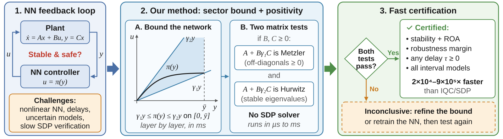
Figure 1: Overview of my framework for Scalable Stability & Robustness Verification of Neural Feedback Systems.
1. Neural Network Bounding
A critical step in verifying neural feedback loops is creating accurate, tractable mathematical models of the neural network’s non-linear behavior. My research focuses on deriving linear “Sector Bounds” that enclose the network’s output.
Software: Both the global and the local sector bounds below are available in my open-source library nnsector, for Python and MATLAB. See the Software page.
Global Sector Bounds
For global stability analysis, I derived a method to calculate Global Sector Bounds for fully connected Feedforward Neural Networks (FFNNs). This method assumes the network has no bias terms (or biases are handled separately), ensuring the origin is an equilibrium point.
- Method: We propagate the sector properties of individual activation functions (like ReLU or Tanh) layer-by-layer through the weight matrices.
- Result: This yields a global linear envelope valid for the entire state space: $$\Gamma_1 x \le NN(x) \le \Gamma_2 x$$ where the bounding matrices are defined as: $$\Gamma_1 = -c^q \left( \prod_{i=1}^{q+1} |W^i| \right), \quad \Gamma_2 = c^q \left( \prod_{i=1}^{q+1} |W^i| \right)$$
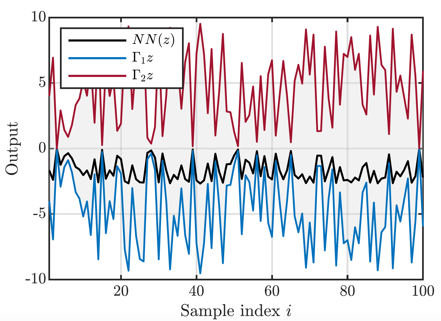
Figure 2: Validation of Global Sector Bounds. The black line represents the neural network output $NN(z)$, which is strictly contained within the linear envelope formed by the lower bound $\Gamma_1 z$ (blue) and upper bound $\Gamma_2 z$ (red) for all 100 random samples.
Performance Comparison
As shown in Table 1, our method computes bounds orders of magnitude faster than IQC-based methods while providing tighter envelopes than standard norm-based approximations.
| Method | Network Architecture | Computation Time (s) | Bounds |
|---|---|---|---|
| Our Method | 10 / 10 / 1 | $2.5 \times 10^{-5}$ | $\pm[2.65, 1.61]$ |
| Our Method | 10 / 15 / 15 / 1 | $2.6 \times 10^{-5}$ | $\pm[2.75, 1.47]$ |
| IQC Method | 10 / 10 / 1 | $0.68$ | — |
| Product of Norms | 10 / 10 / 1 | — | $5.83$ |
| Product of Norms | 10 / 15 / 15 / 1 | — | $6.45$ |
Table 1: Comparison of computation time and bound tightness. (10/10/1 denotes a 3-layer NN with 10, 10, and 1 neurons). Note that IQC does not explicitly provide bounds for the entire NN, and Product of Norms is used only for bound comparison, not stability verification.
Local Sector Bounds
Global bounds can be conservative. To address this, I developed a novel Local Sector Bound formulation.
The construction contains the iteration of two stages as shown in Figure 3. This is the standard procedure used in calculating other NN bounds like CROWN (Wang et al., 2021).
- S1: Propagate sector bounds through the weight matrix and bias.
- S2: Sector-bounding the activations $\phi$ over their input interval.
Iterating S1–S2 from the input to the output yields constant matrices $\gamma_1, \gamma_2$ such that $\gamma_1 y \le \pi(y) \le \gamma_2 y$ for all $y \in \Lambda$.

Figure 3: Schematic illustration of the recursive procedure for computing local sector bounds. We propagate interval bounds layer-by-layer to determine the precise slope matrices $\gamma_1$ and $\gamma_2$.
- Innovation: By restricting the analysis to a specific compact set of inputs, we calculate tighter, input-dependent slope matrices.
- Advantage: These bounds are significantly tighter than norm-based approximations and avoid the affine offsets used in methods like CROWN, making them compatible with robust control frameworks.
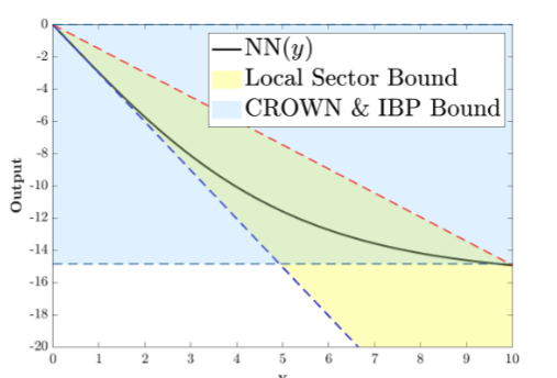
Figure 4a: Comparison of bound structure. Our "Local Sector Bound" (yellow) is structurally different from the standard interval-based bounds used in CROWN/IBP, making it suitable for integrating with positive Aizerman conjecture.
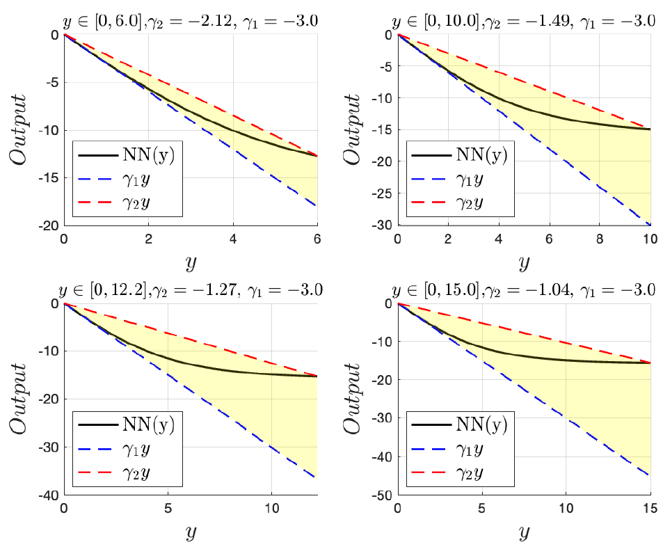
Figure 4b: Visualization of Local Sector Bounds for different input intervals. The yellow region indicates the computed sector, which tightly encloses the neural network's nonlinearity (black line).
2. Stability Verification & Safety
Once the neural network is bounded, I use Control Theory to certify that the closed-loop system (the robot or plant + the neural network) is stable.
Software: The Metzler and Hurwitz stability tests and the region of attraction estimate below are available in my open-source library nnstab, for Python and MATLAB. See the Software page.
Positive Aizerman Framework
My verification pipeline relies on the Positive Aizerman Conjecture. By embedding the bounded neural network into a “Positive Lur’e System” framework, we reduce the complex stability problem to simple linear algebra checks.
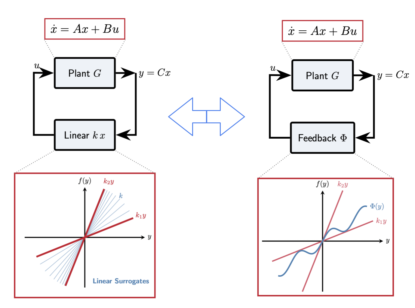
Figure 5: Conceptual overview of the Aizerman Framework. We replace the nonlinear feedback $\Phi$ with linear surrogates $k x$ bounded within the sector $[k_1, k_2]$. If the system is stable for these linear bounds, it guarantees stability for the nonlinear system.
- Efficiency: Instead of solving computationally expensive Linear Matrix Inequalities (LMIs), we simply check if the resulting system matrices are Metzler and Hurwitz.
- Scalability: This approach achieves up to $\approx 10^4\times$ speedup over state-of-the-art methods, enabling verification of larger systems.
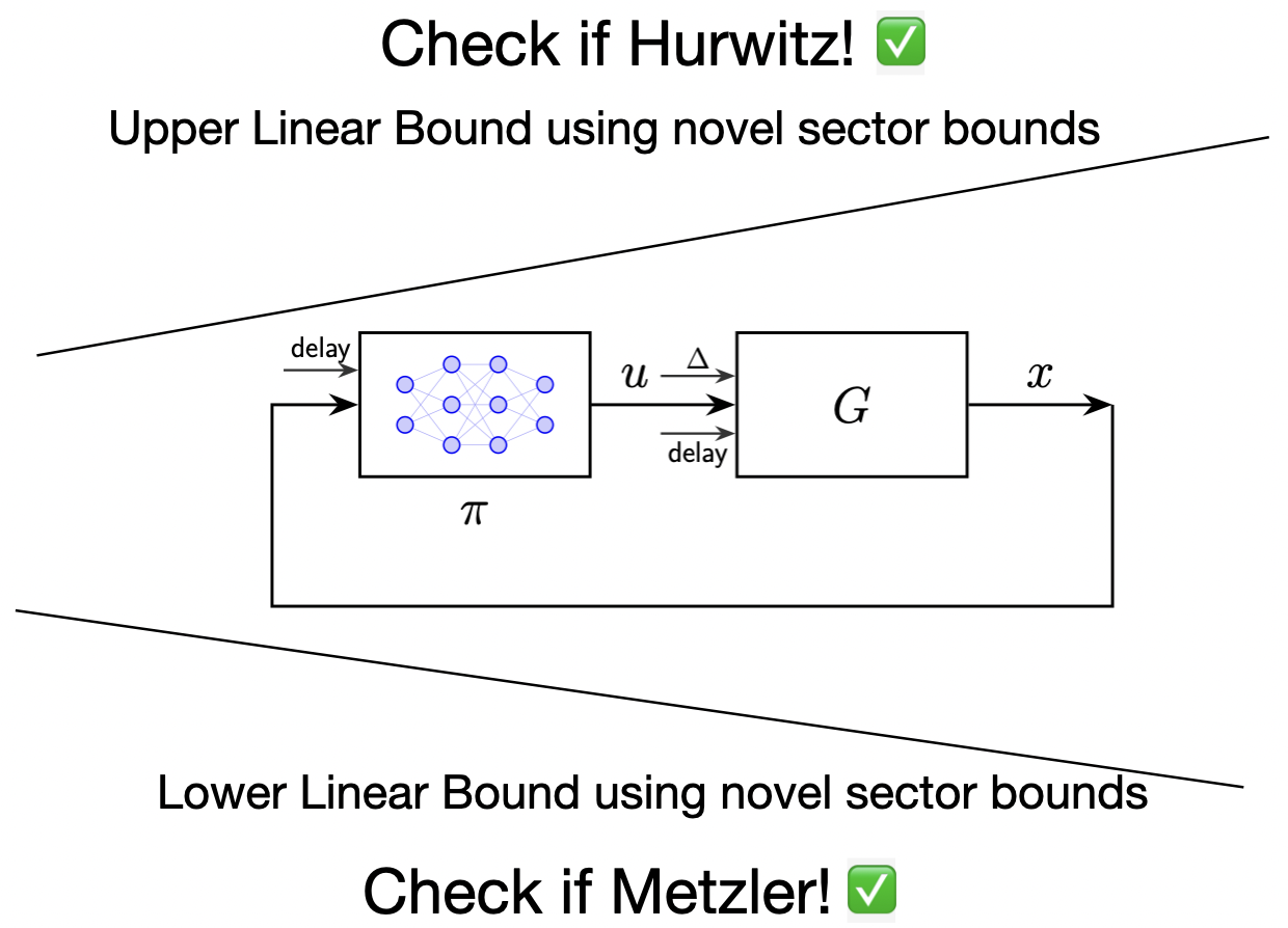
Figure 6: The simplified verification condition. By constructing lower and upper linear bounds using our novel sector method, stability is certified by checking if the lower bound is Metzler and the upper bound is Hurwitz.
Region of Attraction (ROA) Analysis
For systems that are not globally stable, I use the Local Sector Bounds to estimate the Region of Attraction (ROA).
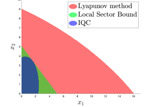
Figure 7: Estimation of the Region of Attraction (ROA). The yellow areas represent the certified safe sets of initial conditions from which the system is guaranteed to converge to the origin, calculated using our local sector bounds.
- Guarantee: We identify a safe set of initial conditions from which the system is guaranteed to converge to equilibrium.
- Performance: Our method certifies larger ROAs than standard IQC-based approaches.
Computational Complexity Comparison
| Operation | Proposed Method (Positive Aizerman) | IQC-based Method (Yin et al., 2021) |
|---|---|---|
| NN bound computation | $O(l_0 q N^2)$ (Matrix Multiplication) | Interval-bound propagation $O(\sum n_i n_{i-1})$ + local slope search $O(n_\phi)$ |
| Stability check | Metzler/Hurwitz tests, $O(n_x^2)$ (One matrix–vector pass) | SDP feasibility with var $P \in \mathbb{S}^{n_x+n_\phi}$ Complexity $O((n_x+n_\phi)^6)$ |
| ROA | Closed-form inequality $Cx_0 \le \frac{\nu_m}{\nu_M} y_{\max}$ | Ellipsoidal ROA via same SDP as stability $O((n_x+n_\phi)^6)$ |
| Scalability (NN params) | Quadratic in NN size ($\sim O(N^2)$) | Cubic in NN size ($\sim O(n_\phi^3)$) via hidden neurons |
| Problem class | LP-like (no SDP), closed-form | Full SDP with IQCs; requires solver |
| Overall Dominant Cost | $O(n_x^3 + N^2)$ | $O((n_x+n_\phi)^6)$ |
3. Risk-Aware Safety Verification (Delays & Uncertainty)
Autonomous systems in the real world face two critical risks: Time Delays (from communication or computation) and Parametric Uncertainty (modeling errors). My research addresses these challenges using two distinct frameworks.
Method A: Positivity-Based Certificates (Scalable)
To address the computational bottlenecks of traditional methods, I developed a delay-independent verification framework based on Positive Systems Theory.
We characterize the uncertain neural feedback system using the following delayed differential inclusion:
\[\dot{x}(t)=\left[\underline{A}_0, \bar{A}_0\right] x(t)+\sum_{i=1}^l\left(\left[\underline{A}_i, \bar{A}_i\right] x\left(t-\tau_i\right)+B_i \,\Phi\!\big(Cx(t-\tau_i)\big)\right)\]- Approach: This model accounts for both parametric uncertainty in the state matrices and the non-linear activation $\Phi$ of the neural network under time-delays $\tau_i$. By enforcing a “Metzler” structure on the interval bounds, we certify stability for all possible delay values.
- Key Result: Robust stability is guaranteed if the lower-bound matrix $\underline{A}$ is Metzler and the resulting interval system is Hurwitz.
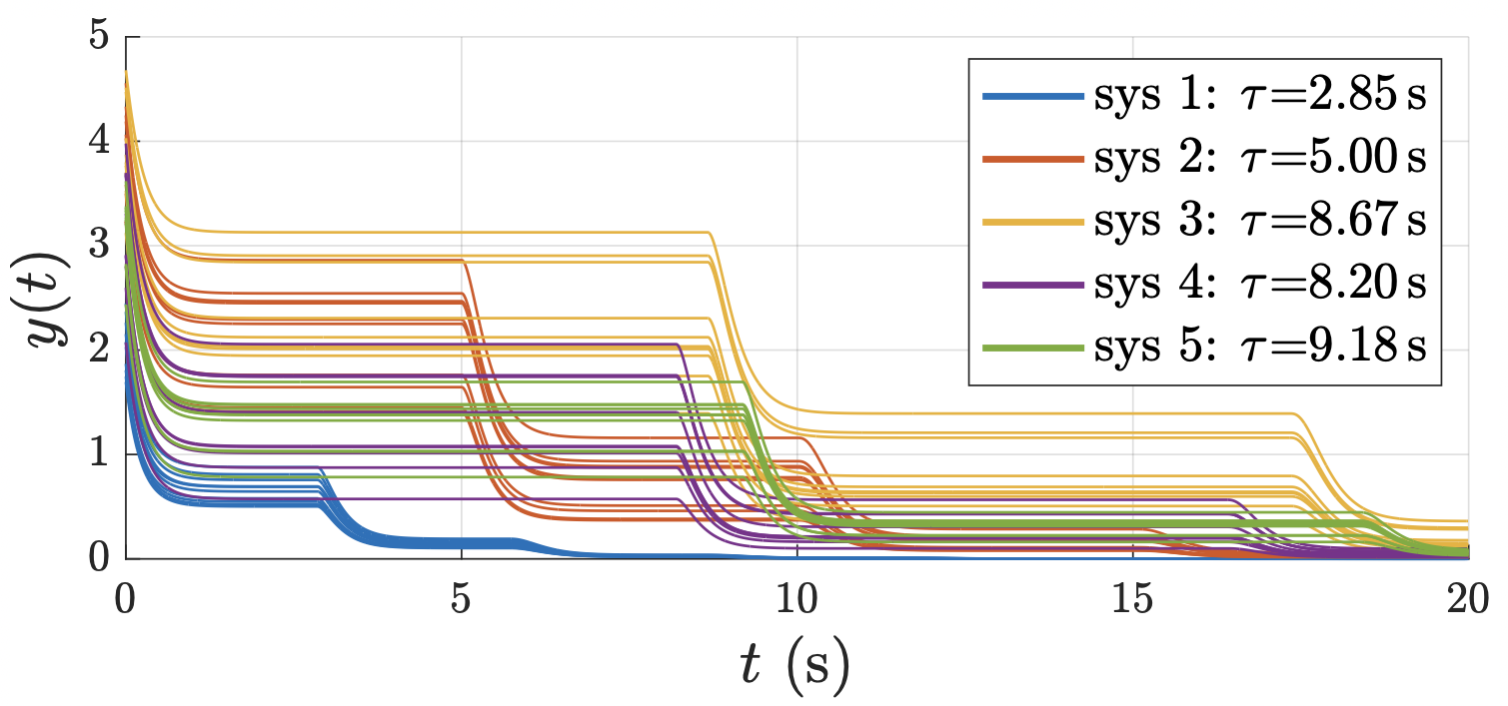
Figure 8: Robustness against structured perturbations and delays. The plot shows sampled trajectories $y(t)$ for systems with varying delays (up to 9.18s), all converging to equilibrium as predicted by the positivity-based certificate.
- Performance: Unlike SDP-based methods that scale cubically with the number of neurons, this algebraic approach maintains efficiency even as the system dimension increases.
Method B: IQC-Based Framework (High-Fidelity)
As a rigorous benchmark, I developed a comprehensive Integral Quadratic Constraint (IQC) pipeline tailored for neural networks with delays and uncertainty.
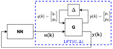
Figure 9: Linear fractional transformation (LFT) model of the NN-feedback-loop with delay and interval uncertainty.
- LFT Modeling: We model the discrete delays and element-wise interval uncertainty as a Linear Fractional Transformation (LFT). This separates the “troublesome” components (uncertainty blocks $\Delta$) from the nominal plant $G$, as shown in the schematic.
- Composite IQCs: We construct a composite IQC filter that combines:
- Delay IQCs: Using delay-line filters to bound the energy of the delay operator.
- Uncertainty IQCs: Using symmetric box multipliers to bound parametric variations.
- Neural Network IQCs: Using sector constraints to bound the nonlinearity.
- Verification: Stability is certified by solving a large-scale Semi-Definite Program (SDP). While computationally heavier than Method A, this framework provides a high-fidelity robust control baseline for AI-enabled systems, ensuring they can handle worst-case scenarios.
4. Crowd Dynamics & Emergency Evacuation
Beyond neural network verification, my research extends to multi-agent systems and public safety. I develop dynamical models to simulate and optimize crowd behavior under high-stress conditions, specifically focusing on active shooter scenarios.
In the absence of an optimized guidance strategy, the crowd (blue agents) relies solely on local repulsive forces. This results in disorganized scattering, increasing vulnerability to the predator (red cross) and yielding higher casualty rates ($K$).
Implementing our tuned parameters ($\alpha=1.625, \lambda=0.71$), the designated guide (green cross) dynamically steers the swarm toward the Safe Zone (green region). This cooperative behavior significantly mitigates casualties by optimizing the trade-off between evasion and evacuation.
The Predator-Swarm-Guide (PSG) Model
We proposed the Predator-Swarm-Guide (PSG) model, a hybrid framework designed to capture the complex interplay between three distinct agent types:
- The Predator: A non-cooperative agent that actively tracks and repels the crowd.
- The Swarm: A multi-agent system governed by social force interactions (pairwise repulsion/attraction) and environmental constraints.
- The Guide: A strategic agent tasked with steering the swarm toward a designated “Safe Zone” while minimizing interaction with the predator.
Key Contributions
- Dynamic Guidance Formulation: We modeled the guide’s trajectory using a weighted objective function parameterized by $\lambda$, which balances the competing goals of “target acquisition” (moving to safety) and “threat evasion” (avoiding the shooter).
- Optimization of Casualty Mitigation: We formulated a nonlinear optimization problem to tune the crowd cohesion parameter ($\alpha_1$) and the guidance weight ($\lambda$). Our results demonstrate that rational cooperation between the guide and the swarm significantly reduces total casualties compared to baseline evacuation methods.
- Continuum Limit Analysis: By deriving the mean-field approximation of the particle model, we provided theoretical characterizations of the crowd’s steady-state spatial distribution, predicting emergent formations such as annular clustering around the threat.
Related Publications
- H. Montazeri Hedesh, M. Siami. “Delay-Independent Safe Control with Neural Networks: Positive Lur’e Certificates for Risk-Aware Autonomy,” American Control Conference (ACC), 2026. [PDF]
- H. Montazeri Hedesh, M. Wafi, M. Siami. “Local Stability and Region of Attraction Analysis for Neural Network Feedback Systems under Positivity Constraints,” IEEE CDC, 2025. [PDF]
- A. Darabi, H. M. Hedesh, M. Siami, M. Sznaier. “Predator-Swarm-Guide Dynamics: A Hybrid Approach to Crowd Modeling and Guidance in Mass Shooting Scenarios,” American Control Conference (ACC), 2024. [PDF]
- H. Montazeri Hedesh, M. Siami. “Ensuring Both Positivity and Stability Using Sector-Bounded Nonlinearity for Systems With Neural Network Controllers,” IEEE Control Systems Letters, 2024. [PDF]